Introduction
What is a Neural Network?
- ReLU = Rectified Linear Unit
| Input | Output | Application | Model |
|---|---|---|---|
| Home Features | Price | Real Estate | NN |
| Ad, User info | Click on ad? 0/1 | Online Advertising | NN |
| Image | Object | Photo Tagging | CNN |
| Audio | Text transcript | Speech Recognition | RNN |
| English | Chinese | Machine Translation | RNN |
| Image, Radar info | Position of other cars | Autonomous Driving | Hybrid |
- Image - convolutional neural network, CNN
- sequence data (temporal data, time series) - recurrent neural network, RNN
- Structured data: database
- Unstructured data: audio, image, text
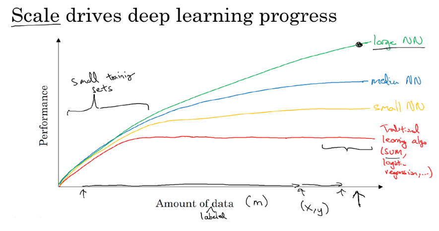
Why is Deep Learning taking off?
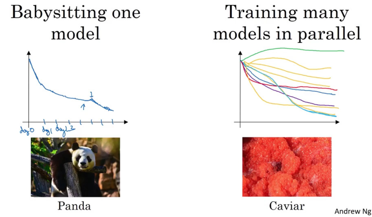
Being able to train a big enough neural network:
- Data: huge amount of labeled data
- Computation
- Algorithms:
- try to make NNs run faster
- e.g. switching from sigmoid to ReLU makes gradient descent algorithm run much faster
Logistic Regression as a Neural Network
- binary classification problem:
$(x,y), x\in \mathbb{R}^{n_x}, y\in\{0,1\}$ $m$training examples:$\{x^{(i)}, y^{(i)}\}_{i=1}^m$
$$ X = \begin{pmatrix} x^{(1)} &x^{(2)} &\cdots &x^{(m)} \end{pmatrix} \in \mathbb{R}^{n_x \times m} $$
$$ y= \begin{pmatrix} y^{(1)} &y^{(2)} &\cdots &y^{(m)} \end{pmatrix} \in \mathbb{R}^{1 \times m} $$
- logistic regression:
Given
$x\in\mathbb{R}^{n_x}$, want$\hat{y}=\Pr(y=1|x)$Output:
$\hat{y}=\sigma(\omega^Tx+b)$, where sigmoid function$\sigma(z)=\frac{1}{1+e^{-z}}$
- if
$z$is large,$\sigma(z)\approx 1$- if
$z$is large negative number,$\sigma(z)\approx 0$$\sigma(0)=0.5$
- cost function:
Given
$\{x^{(i)}, y^{(i)}\}_{i=1}^m$, want$\hat{y}^{(i)}=\sigma(\omega^Tx^{(i)}+b)\approx y^{(i)}$loss(error) function:
$\mathcal{L}(\hat{y},y)=-\left[y\log \hat{y}+(1-y)\log(1-\hat{y})\right]$cost function:
$J(\omega,b)=\frac{1}{m}\sum\limits_{i=1}^m \mathcal{L}(\hat{y}^{(i)}, y^{(i)})=-\frac{1}{m}\sum\limits_{i=1}^m\left[y^{(i)}\log \hat{y}^{(i)}+(1-y^{(i)})\log(1-\hat{y}^{(i)})\right]$
- gradient descent:
$J(\omega,b)$is convex!- algorithm:
repeat{
$\omega\leftarrow \omega - \alpha\frac{\partial}{\partial\omega} J(\omega,b)$
$b\leftarrow b - \alpha\frac{\partial}{\partial b} J(\omega,b)$}
- computation graph:
- forward propagation: compute current loss
- back propagation: compute current gradient
- logistic regression gradient descent: update parameters
One training example:
$z= \omega^Tx+b$
$\hat{y} = a = \sigma(z)$
$\mathcal{L}(a,y)=-(y\log a+(1-y)\log(1-a))$
da:=$\frac{d\mathcal{L}}{da}=-\frac{y}{a}+\frac{1-y}{1-a}$
dz:=$\frac{d\mathcal{L}}{dz}=\frac{d\mathcal{L}}{da}\frac{da}{dz}=\left[-\frac{y}{a}+\frac{1-y}{1-a}\right]a(1-a)=a-y$
dwi:=$\frac{\partial \mathcal{L}}{\partial \omega_i}=x_i\frac{d\mathcal{L}}{dz}$=xi*dz
db:=$\frac{\partial \mathcal{L}}{\partial b}=\frac{d\mathcal{L}}{dz}$=dz
$\omega_i\leftarrow \omega_i - \alpha$dwi
$b\leftarrow b - \alpha$db
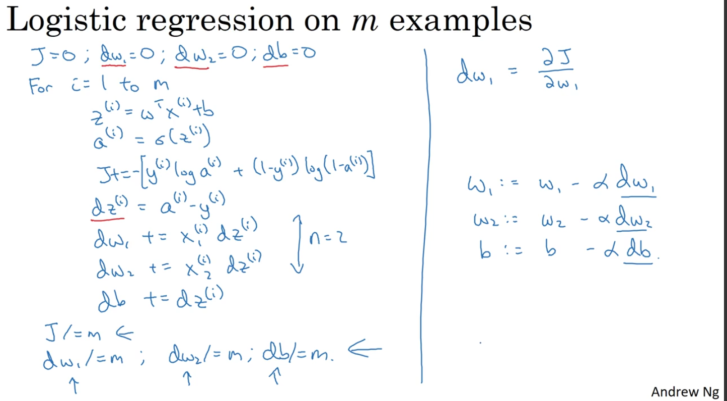
$m$ training examples:
$z^{(i)}= \omega^Tx^{(i)}+b$
$\hat{y}^{(i)} = a^{(i)} = \sigma(z^{(i)})$
$\mathcal{L}(a^{(i)},y^{(i)})=-(y^{(i)}\log a^{(i)}+(1-y^{(i)})\log(1-a^{(i)}))$
$J(\omega,b)=\frac{1}{m}\sum_{i=1}^m \mathcal{L}(a^{(i)},y^{(i)})$
$\frac{\partial J}{\partial\omega_i} = \frac{1}{m}\sum_{i=1}^m\frac{\partial}{\partial\omega_i}\mathcal{L}(a^{(i)},y^{(i)})$
2 for loops: loop over all entries ($m$), loop over all features ($n$)
$\Rightarrow$ vectorization, more efficient!
Vectorization
- Whenever possible, avoid explicit for-loops.
def sigmoid(u):
    return 1/(1 + np.exp(-u))

# X: data, n*m, n = NO. of features, m = NO. of examples
# Y: labels, 1*m
# w: weights, n*1
# b: bias, scalar

# compute activation
A = sigmoid(np.dot(w.T, X) + b)

# cost
J = - np.mean(np.log(A) * Y +  np.log(1-A) *(1-Y))

# back propagation (compute gradient)
m = X.shape[1]
dZ = (A - Y)/m
db = np.sum(dZ)
dw = np.dot(X, dZ.T)

# update params
w -= learning_rate*dw
b -= learning_rate*db
Explanation of Logistic Regression Cost Function
$$ y|x \sim Binom(1, \hat{y}), \hat{y} =\sigma(\omega^Tx+b) $$
$$ \Rightarrow \Pr(y|x)=\hat{y}^y(1-\hat{y})^{1-y}=\begin{cases} 1-\hat{y}, &y=0\newline \hat{y}, &y=1 \end{cases} $$
$$ \Rightarrow \log\Pr(y|x)=y\log\hat{y}+(1-y)\log(1-\hat{y})=-\mathcal{L}(\hat{y},y) $$
Goal: maximize $\Pr(y|x)$ $\Leftrightarrow$ minimize $\mathcal{L}(\hat{y},y)$
Cost on $m$ examples:
maximize $\Pr(\text{labels in training set}) = \prod_{i=1}^n\Pr(y^{(i)}|x^{(i)})$
$\Leftrightarrow$ maximize $\log \prod_{i=1}^n\Pr(y^{(i)}|x^{(i)})=\sum_{i=1}^m\log\Pr(y^{(i)}|x^{(i)})=-\sum_{i=1}^m \mathcal{L}(\hat{y}^{(i)},y^{(i)})$
$\Leftrightarrow$ minimize $J(\omega,b)=\frac{1}{m}\sum_{i=1}^m \mathcal{L}(\hat{y}^{(i)},y^{(i)})$
Image Classification (cat/non-cat) - Python Code
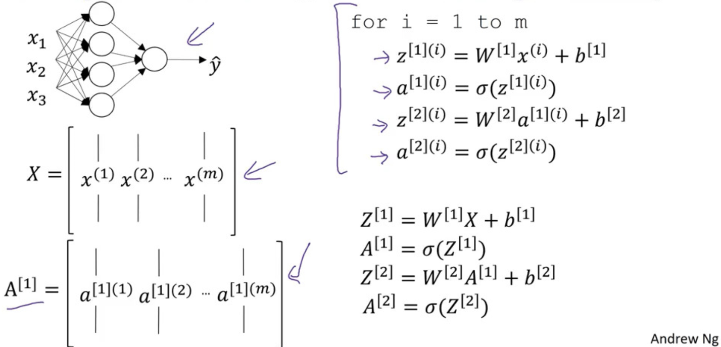
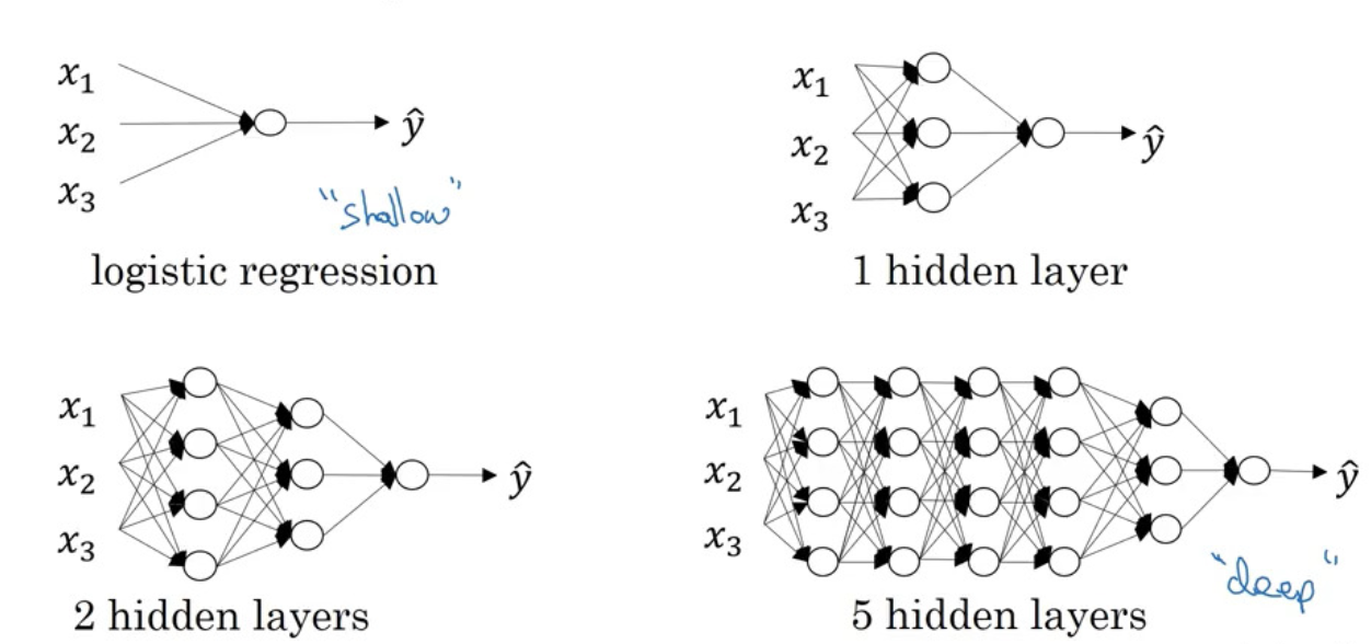
Shallow Neural Network
Forward Propagation
- Neural Network representation:
$k$th layer, with activation function$g^{[k]}$
| Parameters | Dimension |
|---|---|
$W^{[1]}$ |
$(n^{[1]}, n^{[0]})$ |
$b^{[1]}$ |
$(n^{[1]}, 1)$ |
$W^{[2]}$ |
$(n^{[2]}, n^{[1]})$ |
$b^{[2]}$ |
$(n^{[2]}, 1)$ |
$$ A^{[0]} = X, n^{[2]}=1 $$
$$ \text{Forward Propagation }\begin{cases} Z^{[k]} &= W^{[k]}A^{[k-1]} + b^{[k]}, (\text{linear combination}) \newline A^{[k]}&=g^{[k]}(Z^{[k]}), (activation) \end{cases} \ \ k=1,2,\ldots $$
Activation Function
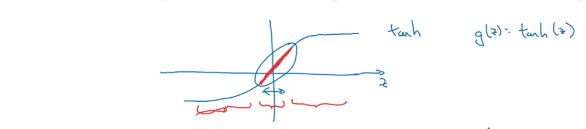
- activation function can be sigmoid, tanh, ReLU, Leaky ReLU…
- for hidden layers, tanh always works better than sigmoid 【the mean of its output is closer to zero, and so it centers the data better for the next layer】
- for output layer of binary classification (0/1), sigmoid may be better
- different layers can have different activation functions
- ReLU is increasingly the default choice (will learn faster)
| function | derivative | |
|---|---|---|
| sigmoid | $\frac{1}{1+e^{-z}}$ |
$g(z)(1-g(z))$ |
| tanh | $\frac{e^z-e^{-z}}{e^z+e^{-z}}$ |
$1-(g(z))^2$ |
| ReLU | $\max(0, z)$ |
$g'(z)=\begin{cases}0, &z<0\newline 1, &z\geq 0\end{cases}$ |
| Leaky ReLU | $\max(0.01z, z)$ |
$g'(z)=\begin{cases}0.01, &z<0\newline 1, &z\geq 0\end{cases}$ |
Gradient Descent
| Single Training Example | m Training Examples |
|---|---|
$dz^{[2]}=a^{[2]}-y$ |
$dZ^{[2]}=\frac{1}{m}(A^{[2]}-y)$ |
$dW^{[2]}=dz^{[2]}a^{[1]T}$ |
$dW^{[2]}=dZ^{[2]} (A^{[1]})^T$ |
$db^{[2]}=dz^{[2]}$ |
$db^{[2]}=np.sum(dZ^{[2]}, axis = 1, keepdims = True)$ |
$da^{[1]}=(W^{[2]})^T dz^{[2]} \circ g^{[1]'}(z^{[1]})$ |
$dZ^{[1]}=(W^{[2]})^T dZ^{[2]} \circ g^{[1]'}(Z^{[1]})$ |
$dW^{[1]}=dz^{[1]}x^T$ |
$dW^{[1]}=dZ^{[1]} X^T$ |
$db^{[1]}=dz^{[1]}$ |
$db^{[1]}=np.sum(dZ^{[1]}, axis = 1, keepdims = True)$ |
Summary
| Forward Propagation | Backward Propagation |
|---|---|
$Z^{[1]}=W^{[1]}X + b^{[1]}$ |
$dZ^{[2]}=\frac{1}{m}(A^{[2]}-Y)$ |
$A^{[1]}=g^{[1]}(Z^{[1]})$ |
$dW^{[2]}= dZ^{[2]} (A^{[1]})^T$$db^{[2]}=np.sum(dZ^{[2]}, axis = 1, keepdims = True)$ |
$Z^{[2]}=W^{[2]}A^{[1]}+b^{[2]}$ |
$dZ^{[1]}=(W^{[2]})^T dZ^{[2]} \circ g^{[1]'}(Z^{[1]})$ 【elementwise product】 |
$A^{[2]}=g^{[2]}(Z^{[2]})=\sigma(Z^{[2]})$ |
$dW^{[1]}= dZ^{[1]} X^T$$db^{[1]}=np.sum(dZ^{[1]}, axis = 1, keepdims = True)$ |
Random Initialization
- If initialize weights and biases with 0: Each neuron in the first hidden layer will perform the same computation. So even after multiple iterations of gradient descent each neuron in the layer will be computing the same thing as other neurons.
- If initialize weights to relative large values ( using the tanh activation for all the hidden units): the inputs of the
tanhto also be very large, thus causing gradients to be close to zero. The optimization algorithm will thus become slow.
Planar Data Classification - Python Code
Deep Neural Network
Notations
$L$: # of layers$n^{[\ell]}$: # of units in layer$\ell$$a^{[\ell]}$: activations in layer$\ell$$a^{[\ell]}=g^{[\ell]}(z^{[\ell]})$
$w^{[\ell]}, b^{[\ell]}$: weights and bias for computing$z^{[\ell]}$
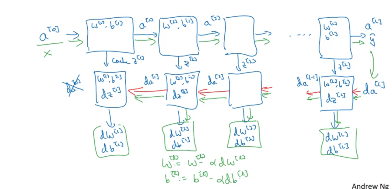
Forward Propagation
Layer $\ell$:
$a^{[0]}:=x$$z^{[\ell]}=W^{[\ell]}a^{[\ell-1]}+b^{[\ell]}$$a^{[\ell]}=g^{[\ell]}(z^{[\ell]})$
(Vectorized) layer $\ell$:
$A^{[0]}:=X$$Z^{[\ell]}=W^{[\ell]}A^{[\ell-1]}+b^{[\ell]}$(numpy broadcasting)$A^{[\ell]}=g^{[\ell]}(Z^{[\ell]})$
Check Dimensions
- shape of
$W^{[\ell]}$and$dW^{[\ell]}$:$(n^{[\ell]}, n^{[\ell-1]})$ - shape of
$b^{[\ell]}$and$db^{[\ell]}$:$(n^{[\ell]}, 1)$ - shape of
$Z^{[\ell]}, A^{[\ell]}, dZ^{[\ell]}, dA^{[\ell]}$:$(n^{[\ell]},m)$
Forward and Backward Functions
layer $\ell$
- Forward:
- input:
$a^{[\ell-1]}$ - output:
$a^{[\ell]}$, cache$z^{[\ell]}$
- input:
- Backward:
- input:
$da^{[\ell]}$ - output:
$da^{[\ell-1]}, dW^{[\ell]}, db^{[\ell]}$ - computation:
- input:
$$
dz^{[\ell]} = da^{[\ell]} * (g^{[\ell]})‘(z^{[\ell]}) \text{ (elementwise product)}\\
dW^{[\ell]} = dz^{[\ell]}a^{[\ell-1]}\\
db^{[\ell]}=dz^{[\ell]}\\
da^{[\ell-1]}=W^{[\ell]T}dz^{[\ell]} \Rightarrow dz^{[\ell]} =W^{[\ell+1]T}dz^{[\ell+1]} * (g^{[\ell]})‘(z^{[\ell]})
$$
$$
\text{Vectorized}: dZ^{[\ell]} = dA^{[\ell]} * (g^{[\ell]})‘(Z^{[\ell]}) \text{ (elementwise product)}\\
dW^{[\ell]} = dZ^{[\ell]}A^{[\ell-1]T}\\
db^{[\ell]}= np.sum(dZ^{[\ell]}, axis=1,keepdims=True)\\
dA^{[\ell-1]}=W^{[\ell]T}dZ^{[\ell]}
$$
Parameters and Hyperparameters
- parameters:
$W^{[\ell]}, b^{[\ell]}$ - hyperparameters:
- learning rate
$\alpha$ - # of iterations
- # of hidden layers
$L$ - # of hidden units
$n^{[\ell]}$ - choice of activation function
- momentum
- minibatch size
- regularizations
- learning rate
Build Deep Neural Network - Image Classification (cat/non-cat) - Python Code
Practical Aspects of Deep Learning
- train/dev/test sets
- traditional rules of thumb ratio: 60/20/20
- big data set: e.g. 98/1/1, 99.5/.4/.1
- mismatched train/test distribution
- guideline: make sure dev and test come from same distribution
- not having a test set is ok (only dev set)
- bias/variance
$\Rightarrow$Basic Recipe:- high bias?
$\rightarrow$bigger network, train longer, NN architecture search - high variance?
$\rightarrow$get more data, regularization, NN architecture search
- high bias?
- no more bias/variance tradeoff:
- pre-deep-learning era: can not just reduce bias or variance without hurting the other
- deep-learning big-data era: a bigger network almost always reduces bias without necessarily hurting the variance so long as you regularize properly; getting more data almost always reduces variance without hurting bias much
Regularization
- reduce variance?
- more data: expensive
- use regularization, prevent overfitting
L2 Regularization
- Cost function
$$ J(W^{[1]},b^{[1]},\ldots,W^{[L]},b^{[L]})=\frac{1}{m}\sum_{i=1}^m\mathcal{L}(\hat{y}^{(i)}, y^{(i)})+\frac{\lambda}{2m}\sum_{\ell=1}^L\Vert W^{[\ell]}\Vert_F^2 $$
where $\Vert\cdot\Vert_F$ is the Frobenius norm.
$dW^{[\ell]}=$(from backprop)$+ \frac{\lambda}{m}W^{[\ell]}$- update:
$W^{[\ell]} := W^{[\ell]} -\alpha dW^{[\ell]}$ $\Rightarrow W^{[\ell]}:=(1-\frac{\alpha\lambda}{m})W^{[\ell]}-\alpha$(from backprop)- L2 regularization = weight decay
- update:
- why regularization reduces overfitting?
- large
$\lambda$$\Rightarrow$$W^{[\ell]}\approx 0$$\Rightarrow$“simpler” network (not zero out hidden units, but some of them have a smaller effect) - e.g., activation
$g = \tanh$, large$\lambda$$\Rightarrow$small$W^{[\ell]}$$\Rightarrow$$z^{[\ell]}=W^{[\ell]}a^{[\ell-1]}+b^{[\ell]}$small$\Rightarrow$$g(z)\approx$linear function$\Rightarrow$nearly linear decision boundary
- large
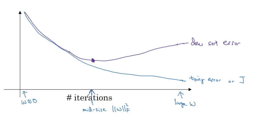
- debugging: with regularization, cost
$J$will not decease monotonically with # of iterations
Dropout Regularization
- Implement Dropout (”Inverted Dropout”)
Illustrate with layer
$\ell=3$keepProb = 0.8 # probability a unit will be kept d3 = np.random.rand(a3.shape) < keepProb a3 *= d3 # elementwise product a3 /= keepProb # ensure the expected value of a3 remains the same
- make predictions at test time: no dropout
- why does dropout work?
- intuition: cannot rely on any one feature, so have to spread out weights
- shrink weights (similar to L2)
- vary
keepProbby layer - cost function is no longer well-defined
Other Regularization Methods
- Data augmentation: e.g. image flip/zoom-in/rotate/distortion
- Early stopping:
- cons: can no longer work on 2 steps of orthogonalization independently
- alternative: L2 regularization (cons: more computationally expensive)
Orthogonalization:
- optimize cost function: gradient descent, …
- not overfit: regularization, …
Speed Up Training
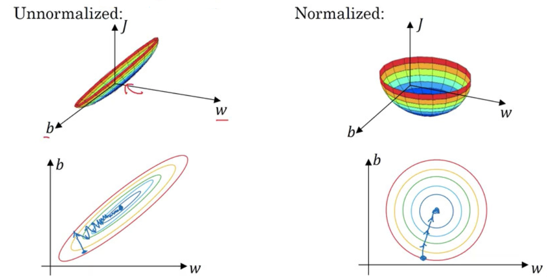
- normalizing training sets
- make sure all features are on similar scale, thus making cost function easier and faster to optimize
- use the same mean/sd to normalized the test set
- weight initialization for deep networks
- partial solution to vanishing/exploding gradients
- use Xavier initialization, …
- can also be tune as hyperparameter
$z=w_1x_1 +w_2x_2 +\cdots + w_nx_n$(omit bias)set
$var(w_i)=\frac{1}{n}$($n=$# of input nodes)W = np.random.randn(node_in, node_out) / np.sqrt(node_in) # relu activation # W = np.random.randn(node_in, node_out) / np.sqrt(node_in/2) # tanh activation # W = np.random.randn(node_in, node_out) / np.sqrt(node_in) # W = np.random.randn(node_in, node_out) / np.sqrt((node_in + node_out)/2)
Debugging of Backpropagation: gradient checking
- take
$W^{[1]},b^{[1]},\ldots,W^{[L]},b^{[L]}$and reshape into a big vector$\theta$ - take
$dW^{[1]},db^{[1]},\ldots,dW^{[L]},db^{[L]}$and reshape into a big vector$d\theta$ - grad check:
for each
$i$: $$ d\theta_{approx}[i]:=\frac{J(\theta_1,\theta_2,\ldots,\theta_i+\epsilon,\ldots)-J(\theta_1,\theta_2,\ldots,\theta_i-\epsilon,\ldots)}{2\epsilon}\approx \frac{\partial J}{\partial \theta_i} $$check $$ \frac{\Vert d\theta_{approx}-d\theta\Vert_2}{\Vert d\theta_{approx}\Vert_2+\Vert d\theta\Vert_2} \approx 0, e.g. < 1e-7 $$
- do not use in training - only to debug
- if algorithm fails grad check, look at components to identify bug
- remember regularization term
- grad check does not work with dropout
- implement grad check without dropout (turn off dropout,
keepProb = 1)
- implement grad check without dropout (turn off dropout,
- run at random initialization; perhaps again after some training
Python Code
Optimization Algorithms
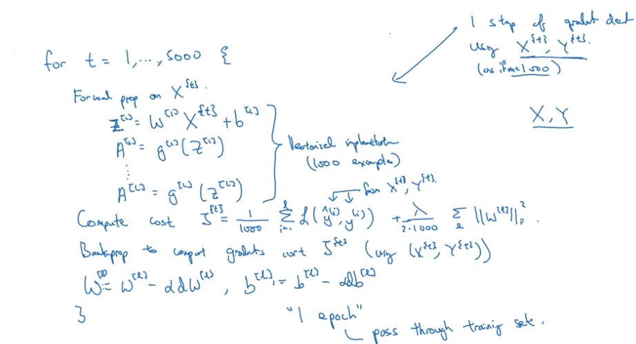
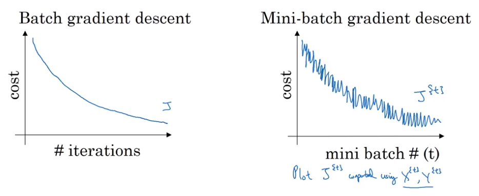
Mini-Batch Gradient Descent
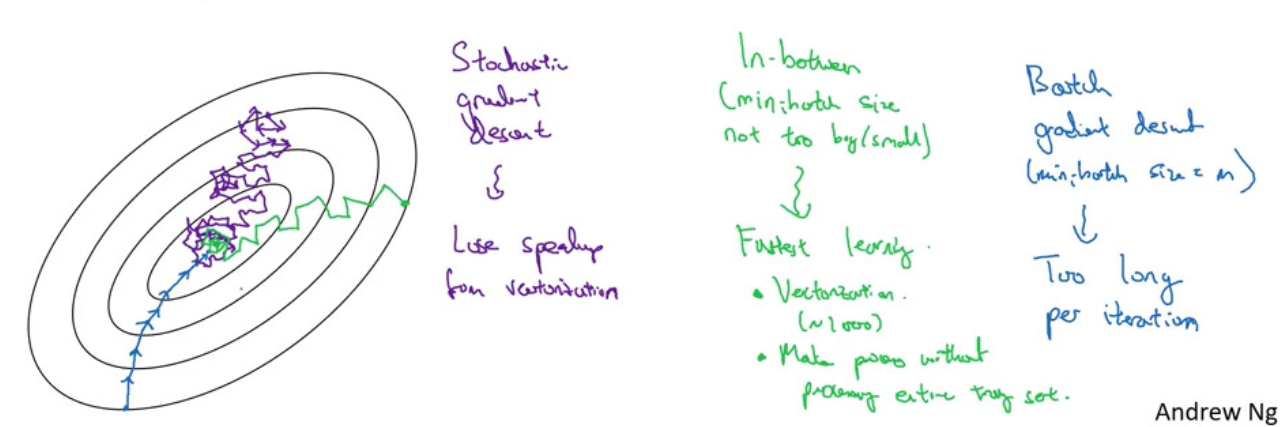
- batch vs mini-batch
- mini-batch
$X^{\{t\}}, y^{\{t\}}$ - mini-batch gradient descent
- choose mini-batch size: hyperparameter
- size =
$m$: batch gradient descent - size = 1: stochastic gradient descent, every example is a mini-batch
- in practice, size between 1 and
$m$- batch gradient descent: too long per iteration
- gradient gradient descent: lose speedup from vectorization
- small training set (
$m\leq 2000$): use batch gradient descent - typical mini-batch size: 64,128,256,512
- make sure mini-batch fits in CPU/GPU memory
- size =
Momentum
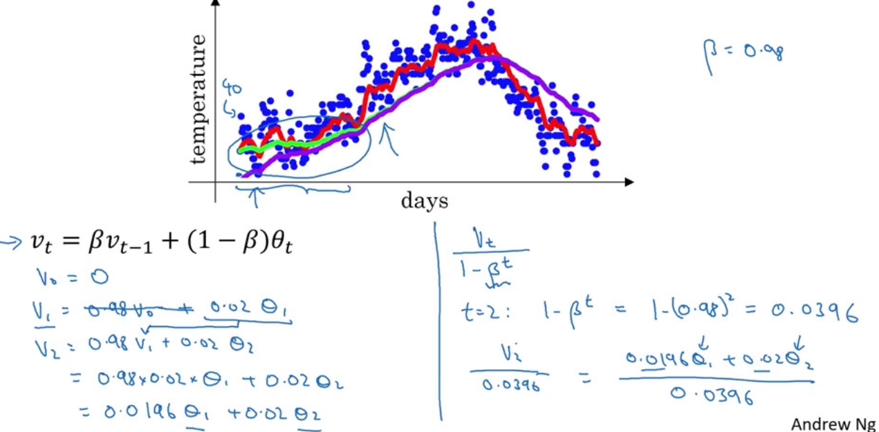
Exponentially Weighted Averages
$$ v_0=0, v_t = \beta v_{t-1}+(1-\beta)\theta_t $$
$$ \Rightarrow v_t = \beta^tv_0 +(1-\beta)\left[ \theta_t + \beta\theta_{t-1} +\ldots \beta^{t-1}\theta_1 \right]=(1-\beta)\sum_{i=0}^{t-1}\beta^i\theta_{t-i} $$
Since
$$
\beta^{\frac{1}{1-\beta}}=\left(1-(1-\beta)\right)^{\frac{1}{1-\beta}}\approx \frac{1}{e},
$$
$v_t\approx$ average of the last $\frac{1}{1-\beta}$ terms of $\theta$’s
$v_{\theta}:=0$repeat{
get next
$\theta_t$
$v_{\theta}:=\beta v_{\theta} + (1-\beta)\theta_t$}
Bias Correction in Exponentially Weighted Averages
Take $v_t := v_t/(1-\beta^t)$
- decrease
$\beta$:- more oscillation
- shift the line to the left
Gradient Descent With Momentum
on iteration
$t$
- compute
$dw,db$on current mini-batch$v_{dw} = \beta v_{dw}+(1-\beta)dw$($v_{dw}$: velocity,$dw$: acceleration,$\beta$: friction)$v_{db} = \beta v_{db}+(1-\beta)db$- update:
$w := w- \alpha v_{dw}, b :=b- \alpha v_{db}$
- hyperparameters:
$\alpha, \beta=0.9$ - no need to do bias correction
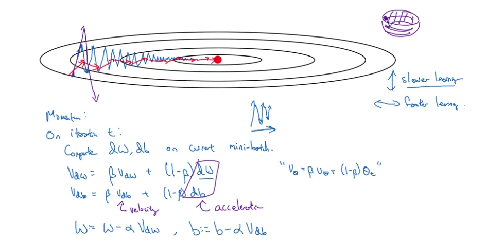
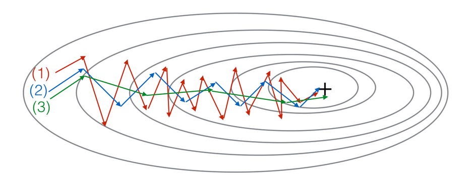
- gradient descent
- with momentum (small
$\beta$) - with momentum (large
$\beta$)
Root Mean Square Prop (RMS Prop)
on iteration
$t$
- compute
$dw,db$on current mini-batch$s_{dw} = \beta s_{dw}+(1-\beta)dw^2$(elementwise square)$s_{db} = \beta s_{db}+(1-\beta)db^2$- update:
$w := w- \alpha \frac{dw}{\sqrt{s_{dw}}+\epsilon}, b :=b- \alpha \frac{db}{\sqrt{s_{db}}+\epsilon}$
- then can use a large learning rate (faster learning), without diverging gradients
$\epsilon$: avoid divide by 0
Adam Optimization Algorithm
- putting it together: momentum + RMS
- adam = adaptive moment estimation
$v_{dw}=0, s_{dw}=0,v_{db}=0,s_{db}=0$on iteration
$t$
- compute
$dw,db$on current mini-batch- momentum:
$v_{dw} = \beta_1 v_{dw}+(1-\beta_1)dw$,$v_{db} = \beta_1 v_{db}+(1-\beta_1)db$- rms:
$s_{dw} = \beta_2 s_{dw}+(1-\beta_2)dw^2$,$s_{db} = \beta_2 s_{db}+(1-\beta_2)db^2$- bias correction:
$v_{dw}^{corrected}=\frac{v_{dw}}{1-\beta_1^t}, v_{db}^{corrected}=\frac{v_{db}}{1-\beta_1^t}$$s_{dw}^{corrected}=\frac{s_{dw}}{1-\beta_2^t}, s_{db}^{corrected}=\frac{s_{db}}{1-\beta_2^t}$- update:
$w := w- \alpha \frac{v_{dw}^{corrected} }{\sqrt{s^{corrected}_{dw}}+\epsilon}, b :=b- \alpha \frac{v^{corrected}_{db}}{\sqrt{s^{corrected}_{db}}+\epsilon}$
- hyperparameters:
$\alpha$: needs to tune$\beta_1$: 0.9 (default)$\beta_2$: 0.99 (default)$\epsilon$: 1e-8 (default)
Learning Rate Decay
- slowly reduce learning rate
- 1 epoch = 1 pass thru the data
- set
$$ \alpha =\frac{1}{1+\text{decay-rate}\times \text{epoch-num}}\alpha_0 $$
- other learning rate decay methods
- exponentially decay:
$\alpha=0.95^{\text{epoch_num}}\alpha_0$ $\alpha=\frac{k}{\sqrt{\text{epoch_num}}}\alpha_0$or$\alpha=\frac{k}{\sqrt{t}}\alpha_0$($t=$mini-batch number)- discrete staircase
- manual decay
- exponentially decay:
Local Optima in Neural Networks
- unlikely to get stuck in a bad local optima
- in nn, most point of 0 gradients are not local optima, but saddle points
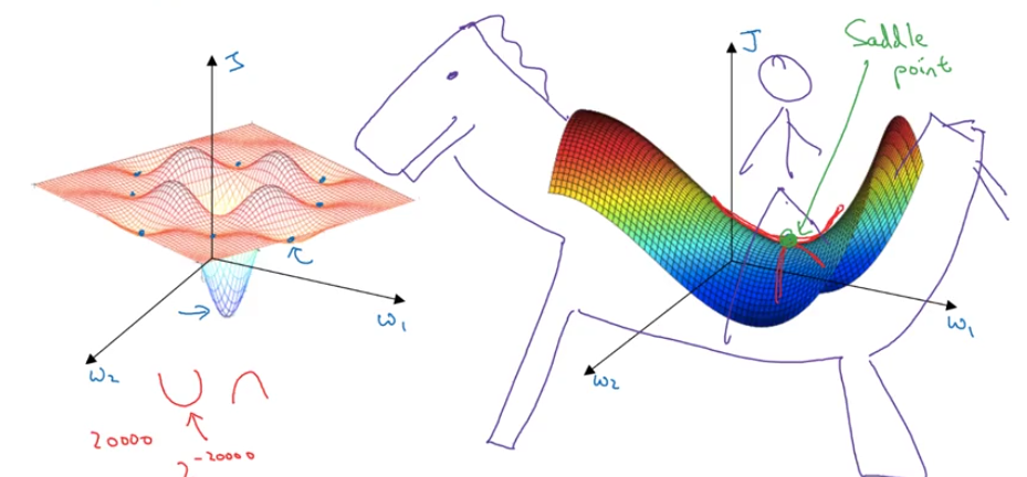
- plateaus can make learning slow
Python Code - Optimization Algorithms
Tuning Process
Hyperparameters
- learning rate
$\alpha$ - momentum
$\beta=0.9$, # of hidden units, mini-batch size - # of layers, learning rate decay
- adam hyperparameters
$\beta_1=0.9, \beta_2=0.99, \epsilon=1e-8$
- try random values, do not use a grid
- coarse to find
- appropriate scale for hyperparameters
- e.g. use log-scale to sample (sample more densely than linear-scale) learning rate
$\alpha$,$1-\beta$
- e.g. use log-scale to sample (sample more densely than linear-scale) learning rate
Hyperparameters Tuning in Practice
Batch Normalization
- normalizing input features can speed up learning
- batch norm: normalize hidden units
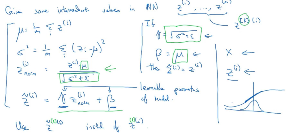
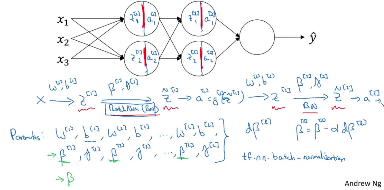
- implementing gradient descent
for
$t=1,2,\ldots, $numMiniBatch
- compute forward prop on
$X^{\{t\}}$- in each hidden layer, use BN to replace
$Z^{[\ell]}$with$\tilde{Z}^{[\ell]}$- use back prop to compute
$dW^{[\ell]}, d\beta^{[\ell]}, d\gamma^{[\ell]}$- update parameters (momentum, RMS prop, adam)
- batch norm reduces covariate shift
- batch norm has slight regularization effect
- batch norm at test time:
- exponentially weighted averages of
$\mu$and$\sigma^2$across mini-batch
- exponentially weighted averages of
Multiclass Classification
Softmax Regression
$C$= # of classes$n^{[L]}=C$- softmax layer:
$$ \text{activation: } t = e^{z^{[L]}},\ a^{[L]}=\frac{e^{z^{[L]}}}{\sum_{j=1}^C t_i} $$
- loss function:
$$ \mathcal{L}(y,\hat{y})=-\sum_{j=1}^Cy_j\log(\hat{y}_j) $$
- cost on the entire training set:
$$ J=\frac{1}{m}\sum_{i=1}^m\mathcal{L}(y^{(i)},\hat{y}^{(i)}) $$
- gradient descent with softmax:
$$ dZ^{[L]}:=\frac{\partial J}{\partial Z^{[L]}}=\hat{y}-y $$
Deep Learning Frameworks
- Caffe/Caffe2
- CNTK
- DL4J
- Keras
- Lasagne
- mxnet
- PaddlePaddle
- Tensorflow
- Theano
- Torch
Choosing Deep Learning Frameworks
- ease of programming (development and deployment)
- running speed
- truly open (open source with good governance)
Signs Recognition with Tensorflow
ML Strategy
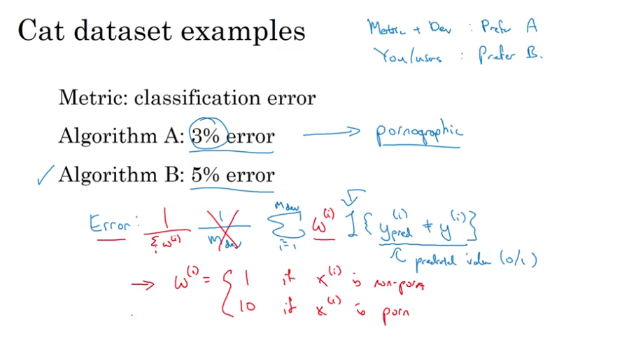
Single Number Evaluation Metric
- precision = PPV = TP/(TP + FP) = 1-FDR
- recall = TPR = TP/P = TP/(TP + FN)
- F1 score = harmonic mean of precision and recall
Satisfying and Optimizing Metric
- accuracy vs running time
- cost = accuracy - 0.5 * running time
- maximize accuracy s.t. running time
$\leq$100ms - accuracy: optimizing
- running time: satisfying
- N metrics:
- pick 1: optimizing
- others: satisfying (threshold)
- e.g. maximize accuracy s.t. false positives
$\leq$threshold
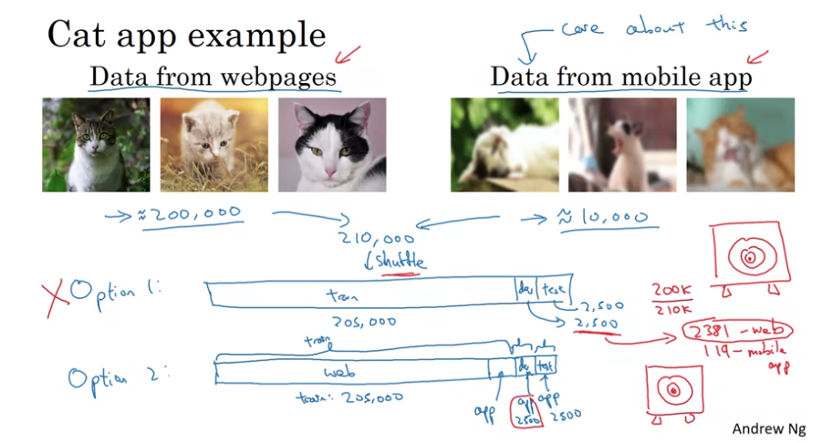
Train/Dev/Test Distributions
- guideline: choose a dev set and test set to reflect data you expect to get in the future and consider important to do well on
- dev set and test set should come from the same distribution
Size of the Dev and Test Sets
- old way of splitting data:
- train/test = 70⁄30
- train/dev/test = 60/20/20
- deep learning
- train/dev/test = 98/1/1
- set your test set to be big enough to give high confidence in the overall performance of your system
- not having a test set is ok, train/dev
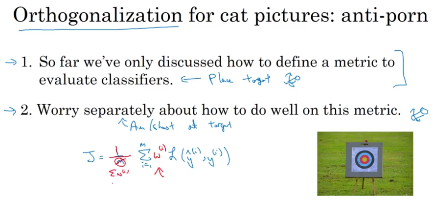
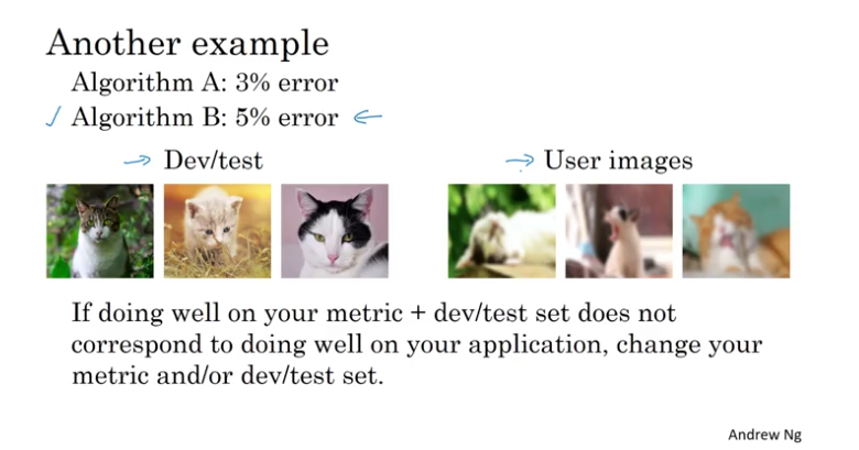
When to Change Dev/Test Sets and Metrics
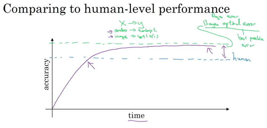
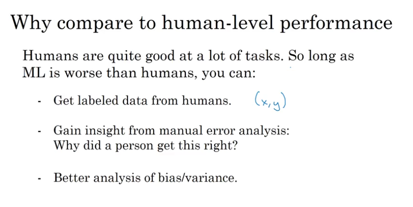
Comparing to Human-Level Performance
- Bayes optimal error
- human-level performance might not be far from Bayes error
- human-level error as a proxy for Bayes error
- avoidable/unavoidable error
- difference between human-level performance & training error: avoidable bias
- difference between training error & dev error: variance
- surpassing human-level performance: (structured data, not natural perception/ lots of data, pattern)
- online advertising
- product recommendations
- logistics (predicting transit time)
- loan approvals
- speech recognition
- some image recognition
- medical: ECG, ….
- two fundamental assumptions of supervised learning
- you can fit the training set pretty well (avoidable bias)
- the training set performance generalized pretty well to dev/test set (variance)
- reduce avoidable bias
- train bigger model
- train longer/ better optimization algo (momentum, RMS prop, Adam)
- NN architecture (CNN, RNN)/ hyperpatameters search
- reduce variance
- more data
- regularization (L2, dropout, data augmentation)
- NN architecture (CNN, RNN)/ hyperpatameters search
Error Analysis
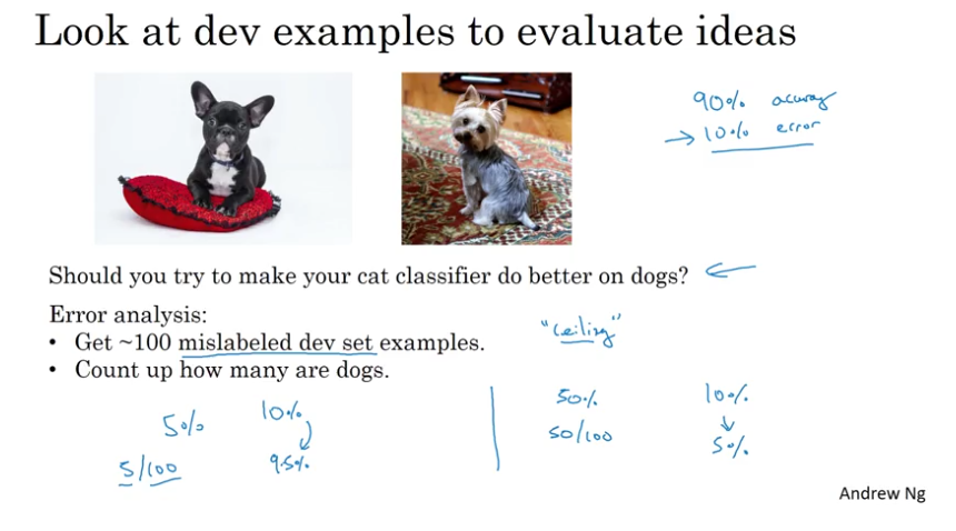
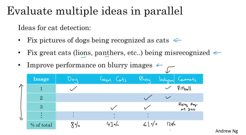
Cleaning Up Incorrectly Labeled Data
- DL algorithms are quite robust to random errors in the training set
- incorrectly labeled data in the dev/test set: add one col in error analysis
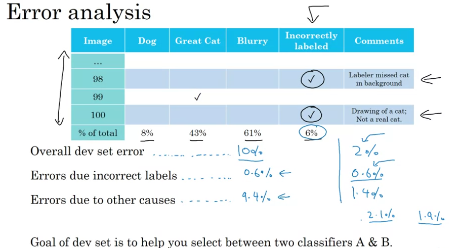
Correcting in correct dev/test set examples
- apply same process to dev and test sets to make sure they continue to come from the same distribution
- consider examining examples your algo got right as well as ones it got wrong
- training and dev/test data may now come from slightly different distributions
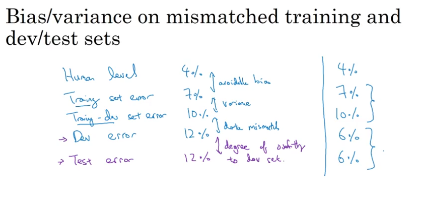
Mismatched Training and Dev/Test Set
- data mismatch problem vs variance problem?
- training-dev set: same distribution as training set, but not used for training
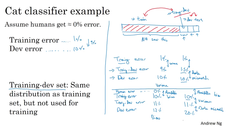
- training error - human-level error = avoidable error
- training-dev error - training error = variance
- dev error - training error = data mismatch
- test error - dev error = degree of overfitting to dev set (larger dev set)
Addressing Data Mismatch
- collect more data similar to dev/test sets
- artificial synthesized data (e.g. speech recognition)
Transfer Learning
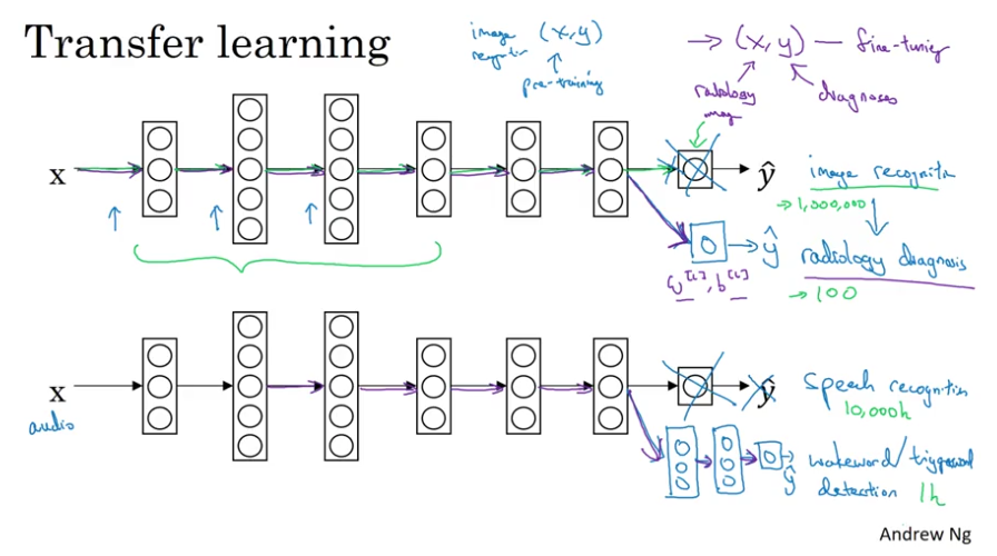
When transfer learning makes sense (Task A $\rightarrow$ Task B)
- Task A and B have the same input
- You have a lot more data for Task A than Task B
- Low level features from A could be helpful for learning B
Multi-task Learning
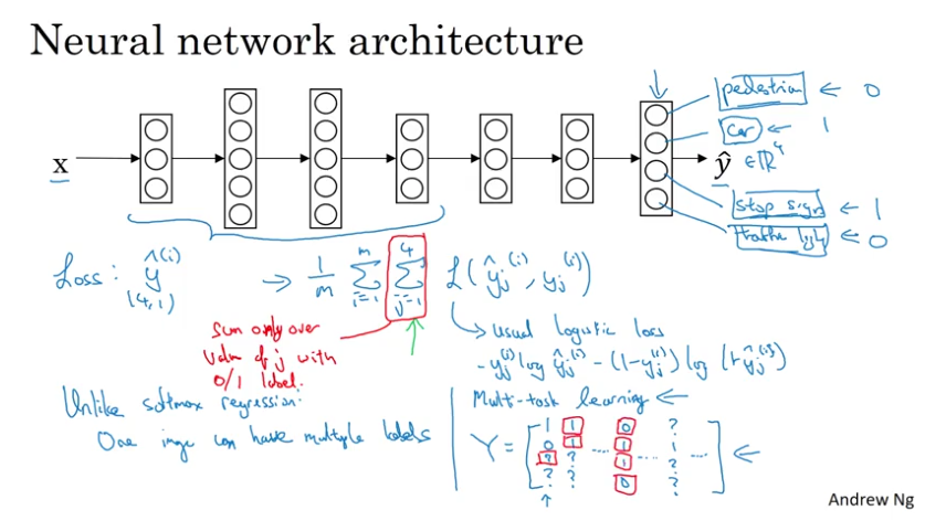
When multi-task learning makes sense
- training on a set of tasks that could benefit from having shared lower-level features
- usually: amount of data you have for each task is quite similar
- can train a big enough nn to do well on all the tasks
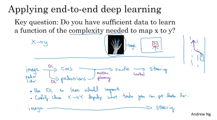
End-to-End Deep Learning
pros of end-to-end deep learning
- let the data speak
- less hand-designing of components needed
cons
- may need large amount of data
- excludes potentially useful hand-designed components