Visualization of Sorting Algorithms
https://www.cs.usfca.edu/~galles/visualization/ComparisonSort.html
https://visualgo.net/bn/sorting
https://www.toptal.com/developers/sorting-algorithms
References
- MIT, 6.006, Introduction to Algorithms, LECTURE 3
- CLRS , Chapter 2
Summary
Best-Case $T(n)$ |
Worst-Case $T(n)$ |
Average-Case $T(n)$? |
Space Complexity | |
|---|---|---|---|---|
| Bubble Sort | $O(n)$ |
$O(n^2)$ |
$O(n^2)$ |
$O(1)$ |
| Selection Sort | $O(n^2)$ |
$O(n^2)$ |
$O(n^2)$ |
$O(1)$ |
| Insertion Sort | $O(n)$ |
$O(n^2)$ |
$O(n^2)$ |
$O(1)$ |
| Merge Sort | $O(n\log n)$ |
$O(n\log n)$ |
$O(n\log n)$ |
$O(n)$ |
| Quick Sort | $O(n\log n)$ |
$O(n^2)$ |
$O(n\log n)$ |
$O(1)$ |
Can We Sort Faster?
- For an array
A[1...n], inversion is a pair(i, j), wherei < jandA[i] > A[j]. - Any algorithm only change the input by adjacent items takes
$\Omega(n^2)$time. - Any comparison-based algorithm takes
$\Omega(n\log n)$time.
Bubble Sort
- Repeatedly swaps adjacent elements which are out of order
- Iterates over the list multiple times, causing larger values to bubble to the end of the list
def bubbleSort(arr):
    n = len(arr)
    for i in range(n-1):
        for j in range(n-i-1):
            if arr[j] > arr[j+1]:
                arr[j], arr[j+1] = arr[j+1], arr[j]
    return arr
- Worst case:
$$ T(n) = (n-1) + (n-2)+\cdots +1=\frac{n(n-1)}{2}=O(n^2) $$
- Bubble sort can be modified to stop early if it finds that the list has become sorted
- List is already sorted (best case):
$O(n)$
def quickBubble(arr):
    n = len(arr)
    unsorted = True
    i = 0
    while unsorted:
        unsorted = False
        for j in range(n-i-1):
            if arr[j] > arr[j+1]:
                arr[j], arr[j+1] = arr[j+1], arr[j]
                unsorted = True
        i += 1
    return arr
Selection Sort
- Each time: minimum computation
- Selection sort improves upon bubble sort by making fewer swaps
- Average case and worst case:
$T(n)=\frac{n(n-1)}{2}=O(n^2)$ - List is already sorted (best case):
$O(n^2)$(Worse than bubble sort!)
def selectionSort(arr):
    n = len(arr)
    for i in range(n-1):
        minIdx = i
        for j in range(i+1, n):
            if arr[j] < arr[minIdx]:
                minIdx = j
        if minIdx != i:
            arr[i], arr[minIdx] = arr[minIdx], arr[i]
    return arr
Insertion Sort
- Maintain the invariant of the prefix of the array (sorted version of those elements)
- Average case and worst case:
$T(n)=\frac{n(n-1)}{2}=O(n^2)$$O(n)$steps (shift key positions)- each step is
$O(n)$comparisons and swaps
- List is already sorted (best case):
$\Theta(n)$ - “Almost sorted” case:
$O(n)$ $O(n\log n)$versus$O(n^2)$: Once the input array length is small or the input array is almost sorted, insertion sort is quicker than merge sort!
def insertionSort(arr):
    n = len(arr)
    for i in range(1, n):
        val, j = arr[i], i
        while j:
            if val < arr[j-1]:
                arr[j], j = arr[j-1], j-1
            else:
                break
        arr[j] = val
    return arr
Binary Insertion Sort
def binarySearch(arr, target, low, high):
    if target < arr[low]:
        return low
    elif target > arr[high]:
        return high + 1

    mid = (low + high)//2

    if arr[mid] == target:
        return mid
    elif arr[mid] > target:
        return binarySearch(arr, target, low, mid-1)
    else:
        return binarySearch(arr, target, mid+1, high)

def insertionSort(arr):
    n = len(arr)
    for i in range(1, n):
        val, j = arr[i], i
        pos = binarySearch(arr, val, 0, i-1)
        while j > pos:
            arr[j], j = arr[j-1], j-1
        arr[pos] = val
    return arr
| Comparison Cost | Swap Cost | |
|---|---|---|
| Insertion Sort | $O(n^2)$ |
$O(n^2)$ |
| Binary Insertion Sort | $O(n\log n)$ |
$O(n^2)$ |
- For numbers, compares
$\approx$swaps - When compares >> swaps (compares are more expensive, e.g. compare records & swap pointers), Binary Insertion Sort gives a better complexity.
| Comparison Cost | Best-Case | Average-Case | Worst-Case |
|---|---|---|---|
| Insertion Sort | $O(n)$ |
$O(n^2)$ |
$O(n^2)$ |
| Binary Insertion Sort | $O(n\log n)$ |
$O(n^2)$ |
$O(n^2)$ |
Inversions
- Running time of Inversion Sort = # of inversions in the array [see Counting Inversions]
PROOF.
Let
$Inv(i)=\# \{ j < i : arr[j] > arr[i]\}$, then $$ \text{# of inversion} = \sum_{i=1}^{n-1} Inv(i) $$ Inversion Sort:for i = 1 to n-1: do$Inv(i)$comparisions and swaps
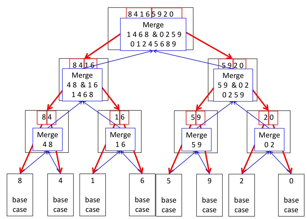
Merge Sort
- Divide and Conquer
- Time complexity:
$O(n\log n)$[See analysis ] - Space complexity:
$O(n)$
def mergeSort(arr):
    n = len(arr)
    # base case
    if n < 2:
        return arr[:]

    m = n//2
    left, right = mergeSort(arr[:m]), mergeSort(arr[m:])

    i = j = 0
    result = []
    for k in range(n):
        if j == n-m or (i < m and left[i] < right[j]):
            result.append(left[i])
            i += 1
        else:
            result.append(right[j])
            j += 1
    return result
- place sentinels
$\infty$at end of each sorted sublists - python list method
append()take amortizedO(1)time
def mergeSort2(arr):
    n = len(arr)
    # base case
    if n < 2:
        return arr[:]

    m = n//2
    left, right = mergeSort(arr[:m]), mergeSort(arr[m:])
    left.append(float('Inf'))
    right.append(float('Inf'))
    i = j = 0
    result = []
    for k in range(n):
        if left[i] < right[j]:
            result.append(left[i])
            i += 1
        else:
            result.append(right[j])
            j += 1
    return result
Merge Sort versus Insertion Sort
- Insertion Sort: in-place; Merge Sort:
$O(n)$auxiliary place 【In-place merge sort】 - Running time:
- Insertion Sort in Python:
$0.2n^2$$\mu s$; in C:$0.01n^2$$\mu s$ - Merge Sort in Python:
$2.2n\log n$$\mu s$ - When n is sufficiently large, Merge Sort in Python beats Insertion Sort in C
- Insertion Sort in Python:
Insertion Sort on Small Arrays in Merge Sort
CLRS, Problem 2-1
Although merge sort runs in
$\Theta(n\log n)$worst-case time and insertion sort runs in$\Theta(n^2)$worst-case time, the constant factor in insertion sort can make it faster in practice for small problem sizes on many machines.Thus, it makes sense to coarsen the leaves of the recursion by using insertion sort within merge sort when subproblems become sufficiently small.
Consider a modification to merge sort in which
$n/k$sublists of length$k$are sorted using insertion sort and then merged using the standard merging mechanism, where$k$is a value to be determined.
- Insertion sort can sort the
$n/k$sublists, each of length$k$in$\Theta(nk)$worst-case time.$$ \frac{n}{k}\times \Theta(k^2) =\Theta(nk) $$
- Merge the sublists in
$\Theta(n\log (n/k))$worst-case time.
- depth of recursion tree:
$\log n - log k + 1=\log(n/k)+1$- merge:
$\Theta(n)$- Thus the modified algorithm runs in
$\Theta(nk + n\log(n/k))$time. If$k=O(\log n)$, the modified algorithm has at most the running time of merge sort in terms of$\Theta-$notation.- Choice of
$k=k(n)$in practice: minimize$$ f(n) = Ank(n) +Bn\log\left(\frac{n}{k(n)}\right) $$
Timsort
Python uses an algorithm called Timsort:
Timsort is a hybrid sorting algorithm, derived from merge sort and insertion sort, designed to perform well on many kinds of real-world data. It was invented by Tim Peters in 2002 for use in the Python programming language. The algorithm finds subsets of the data that are already ordered, and uses the subsets to sort the data more efficiently. This is done by merging an identified subset, called a run, with existing runs until certain criteria are fulfilled. Timsort has been Python’s standard sorting algorithm since version 2.3. It is now also used to sort arrays in Java SE 7, and on the Android platform.
Quick Sort
- Randomized algo
from random import randint

def partition(arr, L, R):
    pivot = arr[L]
    i = L + 1
    for j in range(i, R + 1):
        if arr[j] < pivot:
            arr[j], arr[i] = arr[i], arr[j]
            i += 1
    arr[L], arr[i - 1] = arr[i - 1], arr[L]
    return i - 1

def quickSortHelper(arr, L, R):
    if R - L < 1:
        return arr
    pos = randint(L, R)
    arr[L], arr[pos] = arr[pos], arr[L]
    pos = partition(arr, L, R)
    quickSortHelper(arr, L, pos - 1)
    quickSortHelper(arr, pos + 1, R)

def quickSort(arr):
    return quickSortHelper(arr, 0, len(arr) - 1)