Linear Regression with One Variable
$X$: space of input values,$Y$: space of output valuestraining set
$\{(x^{(i)}, y^{(i)})\}_{i=1}^N$goal: given a training set, to learn a function
$h : X \rightarrow Y$so that$h(x)$is a “good” predictor for the corresponding value of$y$. For historical reasons, this function$h$is called a hypothesis.$h(x)=h_{\theta}(x) = \theta_0 + \theta_1 x$cost function (squared error function, or mean squared error, MSE):
$$ J(\theta_0, \theta_1)= \frac{1}{2N}\sum _{i=1}^N \left(\hat{y}^{(i)} -y^{(i)} \right)^2 =\frac{1}{2N}\sum _{i=1}^N \left(h(x^{(i)}) - y^{(i)}\right)^2 $$
To break it apart, it is $\frac{1}{2} \bar{x}$ where $\bar{x}$ is the mean of the squares of $h_\theta (x_{i}) - y_{i}$ , or the difference between the predicted value and the actual value.
The mean is halved $\left(\frac{1}{2}\right)$ as a convenience for the computation of the gradient descent, as the derivative term of the square function will cancel out the $\frac{1}{2}$ term.
- optimization: minimize
$J(\theta_0, \theta_1)$w.r.t parameters$(\theta_0, \theta_1)$ - Gradient Descent:
Outline:
- Initialize
$\theta_0, \theta_1$- Keep changing
$\theta_0, \theta_1$to reduce$J(\theta_0, \theta_1)$until we hopefully end up at a minimum
Algorithm:
repeat until convergence{
$\theta_j \leftarrow \theta_j -\alpha\frac{\partial}{\partial \theta_j}J(\theta_0, \theta_1),\ \ \ j=0,1$}
$\alpha$: learning rate (step size)
Correct: simultaneous update
$temp0 \leftarrow \theta_0 -\alpha\frac{\partial}{\partial \theta_0}J(\theta_0, \theta_1)$
$temp1 \leftarrow \theta_1 -\alpha\frac{\partial}{\partial \theta_1}J(\theta_0, \theta_1)$
$\theta_0 \leftarrow temp0 $
$\theta_1 \leftarrow temp1 $
Incorrect: WHY?
$temp0 \leftarrow \theta_0 -\alpha\frac{\partial}{\partial \theta_0}J(\theta_0, \theta_1)$
$\theta_0 \leftarrow temp0 $
$temp1 \leftarrow \theta_1 -\alpha\frac{\partial}{\partial \theta_1}J(\theta_0, \theta_1)$
$\theta_1 \leftarrow temp1 $
- learning rate
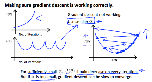
$\alpha$:- too small, gradient descent can be slow
- too large, gradient descent may fail to converge, or even diverge
- as we approach a local minimum, gradient descent will automatically take smaller steps, even with fixed learning rate
- apply gradient descent to linear regression:
$$ \frac{\partial}{\partial \theta_j}J(\theta_0, \theta_1) =\frac{\partial}{\partial \theta_j}\frac{1}{2N}\sum _{i=1}^N \left(h(x^{(i)}) - y^{(i)}\right)^2= \begin{cases} \frac{1}{N}\sum _{i=1}^N \left(h(x^{(i)}) - y^{(i)}\right), & j=0\newline \frac{1}{N}\sum _{i=1}^N \left(h(x^{(i)}) - y^{(i)}\right)x^{(i)}, & j=1 \end{cases} $$
- cost function of linear regression is convex
$\Rightarrow$no local mimina - Batch Gradient Descent: each step of gradient descent uses all the training examples
Multivariate Linear Regression
- notations:
$p$: # of features$\mathbf{x}^{(i)}$: input of$i$th training example$x^{(i)}_j$: value of feature$j$in$i$th training example
- hypothesis: define
$x_0^{(i)}=1, \forall i$
$$ h_{\theta}(\mathbf{x}) =\mathbf{\theta}^T \mathbf{x} = \begin{pmatrix} \theta_0 &\theta_1& \cdots& \theta_p \end{pmatrix} \begin{pmatrix} x_0\newline x_1\newline \vdots\newline x_p \end{pmatrix} $$
- cost function:
$$ J(\mathbf{\theta}) = \frac{1}{2N}\sum_{i=1}^N\left(h(\mathbf{x}^{(i)})-y^{(i)}\right)^2 $$
- Gradient Descent:
Algorithm:
repeat until convergence{
$\theta_j \leftarrow \theta_j -\alpha\frac{\partial}{\partial \theta_j}J(\mathbf{\theta})=\theta_j -\alpha\frac{1}{N}\sum _{i=1}^N \left(h(\mathbf{x}^{(i)}) - y^{(i)}\right)x^{(i)}_j$} (simultaneously update for
$j=0,1,...,p$)
$\alpha$: learning rate (step size)
Gradient Descent in Practice
Feature Scaling
- idea: make sure features are on a similar scale, i.e. approximately
$[-1, 1]$range
Gradient Descent will descent slowly on large ranges, and so will oscillate inefficiently down to the optimum when the variables are very uneven.
Feature scaling can speed up Gradient Descent.
- mean normalization: replace
$x_i$with$x_i-\mu_i$to make features have aproximately 0 mean
$$ x_i \leftarrow \frac{x_i-\mu_i}{s_i}, s_i \text{ range or SD} $$
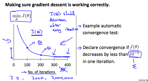
Learning Rate
- fix
$\alpha$, plot$J(\mathbf{\theta})$versus no. of iterations$\alpha$too small: slow convergence$\alpha$too large: may not converge


Vectorization
- compute cost:
$$ J(\theta) = \frac{1}{2N}(X\theta-y)^T(X\theta-y) $$
import numpy as np
# residual
resid = np.dot(X, theta) - y
cost = np.mean(resid ** 2)/2
- gradient descent:
$$
\theta_j \leftarrow \theta_j -\alpha\frac{\partial}{\partial \theta_j}J(\mathbf{\theta})\\
\Rightarrow \mathbf{\theta} \leftarrow \mathbf{\theta}-\alpha\frac{d}{d\mathbf{\theta}}J(\mathbf{\theta})=\mathbf{\theta}-\frac{\alpha}{N}X^T (X\theta -y)
$$
theta -= learning_rate/m*np.dot(X.T, resid)
Normal Equation
- design matrix:
$$ X_{N\times(p+1)}=\begin{pmatrix} \mathbf{1} &\mathbf{x}_1 &\cdots &\mathbf{x}_p \end{pmatrix} $$
where $$ \mathbf{x}_j = \begin{pmatrix} x_j^{(1)}\newline x_j^{(2)}\newline \vdots\newline x_j^{(N)} \end{pmatrix} $$
- output:
$$ \mathbf{y}=\begin{pmatrix} y^{(1)}\newline y^{(2)}\newline \vdots\newline y^{(N)} \end{pmatrix} $$
$$ \Rightarrow \hat{\mathbf{\theta}} = (X^TX)^{-1}X^T\mathbf{y} $$
| Gradient Descent | Normal Equation |
|---|---|
| need to choose learning rate | no need to choose learning rate |
| need feature scaling | no need to do feature scaling |
| many iterations | no need to iterate |
$O(kp^2)$, $k$ is the no. of iterations |
$O(p^3)$, need to compute $(X^TX)^{-1}$ |
works well when $p$ is large |
slow if $p$ is very large |
Normal Equation Noninvertibility
- what is
$X^TX$is noninvertible? (singular/degenerate)- redundant features (linearly dependent)
- too many features (
$N\leq p$)$\Rightarrow$delete some features, or use regularization
- pseudo-inverse